Tag Archives: SAS

ORA-00972 Error with SQL Pass-Through in SAS

If you are using explicit pass-through syntax in SAS, you can run into problems when naming conventions in the native database are different from those in SAS. For example, this can happen when SAS allows more characters for an identifier than Oracle does. I ran the following statements in SAS to pull some pharmacy claims and got an error in my log:

proc sql;
connect to oracle (path=”pathname” user=xxxxxxx password=xxxxxxxx);
create table sasuser.thrx_rx_claim_2012 as
  select * from connection to oracle
    (
    select a.indiv_enterprise_id
    ,b.clm_pd_dt
    ,b.svc_beg_dt
    ,b.svc_end_dt
    ,b.elgbl_chrg_amt
    ,b.mail_retl_cd
    ,b.new_prscrptn_ind
      from c31497.thrx_id_elig_rsk_cens_dedup_2012 a
      left join ccdm_mart.clm_svc b on a.indiv_enterprise_id=b.indiv_enterprise_id
        where svc_beg_dt >= to_date(’01/01/2012′,’mm/dd/yyyy’)
        and svc_beg_dt <= to_date(’12/31/2013′,’mm/dd/yyyy’)
        and CVRD_AMT<>NOT_COVRD_AMT
        and clm_frmt_ty=’RX’
    )
;
quit;

Here is the error I received in the log:
ORA-00972: identifier is too long

An identifier can refer to a table name or a column (variable) name. In this case the table name thrx_id_elig_rsk_cens_dedup_2012 in the FROM statement is exactly 32 characters, which is the maximum allowable in SAS. However, Oracle gives you a maximum of 30 characters, so the query will not run.

Case-Sensitive Schema in a SAS Libname Statement

This is a minor annoying issue that had been bothering me for a few years (!) and was finally resolved with a ticket to SAS Tech Support. I have several libname statements that I have been using to connect to DB2 databases. In the past, the libname statements all ran successfully, and I was able to query the tables in the databases. However, when I tried to view the tables under my assigned libraries in the SAS Explorer window by clicking on the libname, the libraries appeared empty. This was irritating since I either had to use another tool if I wanted to browse the tables and look at the actual data, or rely on Proc Contents.

The answer to the problem turns out to be that some schemas are case-sensitive. SAS Tech Support suggested trying the following libname statements:

libname CRDM1 db2 dsn=crdm schema=appdm uid=xxxxx pwd=xxxxxx sql_functions=all dbindex=yes;

libname CRDM2 db2 dsn=crdm schema=”appdm” uid=xxxxx pwd=xxxxxx sql_functions=all dbindex=yes;

libname CRDM3 db2 dsn=crdm schema=APPDM uid=xxxxx pwd=xxxxxx sql_functions=all dbindex=yes;

libname CRDM4 db2 dsn=crdm schema=”APPDM” uid=xxxxx pwd=xxxxxx sql_functions=all dbindex=yes;

The first and second libname statements didn’t display the tables, but the last two with the schema in all CAPS both worked.

Model Evaluation: Explaining the Cumulative Lift Chart

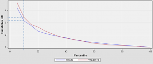
I recently developed a model for a client in which the goal was to identify at-risk customers with chronic conditions to target for outreach in a health coaching program. By targeting the customer for outreach, we hoped to improve the patient’s health, medication adherence, and avoid costly emergency room visits and inpatient admissions. In order to explain how effective the model was, I used a cumulative lift chart created in SAS Enterprise Miner (click the image below to enlarge):

lift_chart

The x-axis shows the percentile and the y-axis shows lift. Keep in mind that the default (no model), is a horizontal line intersecting the y-axis at 1. If we contact a random 10% of the population using no model, we should get 10% of the at-risk customers by default; this is what we mean by no lift (or lift=1). The chart above shows that using the given model we should be able to capture 32-34% of the at-risk customers for intervention if we contact the customers with risk scores in the top 10 percentile (shown by the dashed line). That is more than 3 times as many as if we use no model, so that is our “lift” over the baseline. Here is another example using te same chart: we can move to the right on the lift curve and contact the top 20% of our customers, and we would end up with a lift of about 2.5. This means that by using the model, we could capture about 50% of the at-risk customers if we contact just 20% of them.

The cumulative lift chart visually shows the advantage of using a predictive model to choose who to outreach by answering the question of how much more likely we are to reach those at risk than if we contact a random sample of customers.

Checking the Match in a Matched Case-Control Study

Sometimes we wish to conduct a study in which we take a population of interest (the treatment group) and match each case to a similar individual sampled from the population which is not undergoing the treatment (the control group). The goal is to find out whether the outcome we wish to measure after treatment is significantly different for each population. This is known as an individually matched case-control study. This post will focus on checking that the matched case population is similar to the control population.

For example, say that we want to find out if providing an incentive to individuals in the treatment group will influence their behavior. We might match on the following variables: medical condition, gender, geographic area, age, risk score, number of office visits in the past 12 months, and total medical cost (TMC) in the past 12 months. Some of these we would want an exact match for (the first 3 variables in this example), whereas the last 4 variables we would match within a given range.

After we run the match, we want to check that the characteristics for the treatment group are similar to those of the control group — that the population means are not significantly different for the continuous variables such as TMC. In order to check this, we first want to test for normality. Whether or not the variable is normally distributed will determine which kind of test we run to see if there is a significant difference between the two groups.

To test normality for the variable TMC, we can use PROC UNIVARIATE as follows:

proc univariate data=work.testdata normal plot;
var TMC;
qqplot TMC /normal(mu=est sigma=est color=red L=1);
run;

This will give you a boxplot and a q-q plot, and the NORMAL option will also give you some normality tests, including Shapiro-Wilk (good for sample sizes < 2000). For normality, you want the mean and the median to be close together on the box plot, a reasonably symmetric distribution (skew close to zero), a relatively straight line for the q-q plot, and the p-values on the normality test results should be > 0.05. If the Shapiro-Wilk W value is close to 1, this also indicates that the data is normal. If p-values are less than 0.05 (alpha), that means you reject the null hypothesis that the distribution is normal and proceed with non-parametric testing.

Assuming your distribution is normal, you would run a paired t-test to see if TMC is similar for both populations (in this example, “study_group” is a flag variable that indicates whether the observation is in the treatment/study group or the control group):

proc ttest data=work.testdata;
paired TMC*study_group;
run;

The null hypothesis is that there is no statistically significant difference between the two groups, so you would want to see a large p-value here (>0.05). This would indicate that our two populations are well-matched on this variable.

However, it is unlikely that TMC is normally distributed, so you would probably end up using the NPAR1WAY procedure instead, with the Wilcoxon test (again, the null hypothesis says that the means are equal, so we want large p-values since we want to accept the null hypothesis):

proc npar1way data=work.testdata wilcoxon;
class study_group;
var TMC;
run;

The tests shown above have all been for continuous variables. Alternatively, if you wanted to test a discrete variable such as gender, you could use PROC FREQ with a chi square test to ensure that gender is independent of the study_group variable:

proc freq data=work.testdata;
tables study_group*male / chisq fisher;
run;
SAS Survey Procedures: PROC SURVEYLOGISTIC vs. PROC LOGISTIC Output

In a previous post, I talked about complex survey designs and why analysis of such survey data requires the use of SAS survey procedures. PROC SURVEYREG and PROC SURVEYLOGISTIC have some of the same options available for output/diagnostics as do their non-survey counterparts, PROC REG and PROC LOGISTIC. Default output includes fit statistics (R squared, AIC, and Schwartz’s criterion), chi-squared tests of the global null hypothesis, degrees of freedom, and coefficient estimates for each parameter along with standard error of coefficient estimates and p-values. PROC SURVEYLOGISTIC also includes odds ratio point estimates and 95% Wald confidence intervals for each input parameter, as does PROC LOGISTIC.

The survey procedures are more limited in some ways, though. For example, PROC LOGISTIC can use an option such as stepwise selection to restrict the output to only predictors with significance above a certain level; there is also an option to rank those predictors. These options do not work with PROC SURVEYLOGISTIC, which makes the output more unwieldy with a large number of predictors. Most notably in terms of differences, PROC LOGISTIC automatically outputs a chi-squared test of the residuals for each input variable; however, any analysis of residuals is irrelevant for the survey procedures since assumptions of normality and equal variance are not applicable due to survey design. Tabled residuals are not output at all for the survey procedures, although covariance matrices are available for both as a non-default option. Similarly, influential observations/outliers are also not analyzed due to the use of person weights. As long as we use person weights, we would get the same coefficients with a regular PROC REG as we would with PROC SURVEYREG, but standard error estimates would be different and predictor significance could also vary.