Tag Archives: normality tests

Testing for Normality in R

In the post that follows, I will show how to test for normality in R, both by visual examination of box plots and q-q plots, and also by using the Shapiro-Wilk normality test. R code and output are included for all steps. The first step is to read in the data file, which already includes the variable “income.” I then calculate the log transformation of income and add it to the data set:

cir<-read.table(“CIR.txt”,header=TRUE)
cir<-cbind(cir,logincome=log(cir$income))

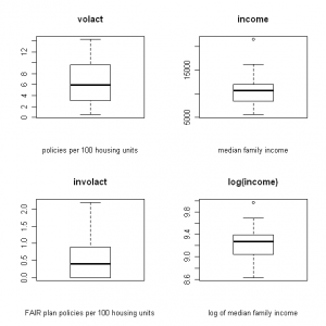
Next I create four boxplots, naming each and labeling the x axis. I wish to display all four on a single page in a 2 x 2 matrix (click the images below to enlarge):

layout(matrix(1:4,2,2))
boxplot(cir$volact,xlab=”policies per 100 housing units”,main=”volact”)
boxplot(cir$involact,xlab=”FAIR plan policies per 100 housing units”,main=”involact”)
boxplot(cir$income,xlab=”median family income”,main=”income”)
boxplot(cir$logincome,xlab=”log of median family income”,main=”log(income)”)

boxplot_1

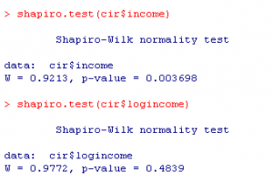
At a glance, the volact box plot looks the most symmetrical, from which we can infer normal distribution. Involact and income appear less normally distributed than volact. The log (income) box plot looks a little better than the income box plot, but it is difficult to say for sure. We can verify this by running the Shapiro-Wilk normality test on each variable, where the null hypothesis assumes normality (results shown below for income vs. log (income)).
normality_test_r

For income, the normality test gives small W and p-values which would cause us to reject H0 (normal distribution) at alpha=0.05 and conclude the distribution of income is not normal. Results for the transformation log (income) show normal distribution, which we can conclude from the large p-value and larger W. This makes sense, since we know that income is seldom normally distributed; the distribution is typically skewed by very high outliers.

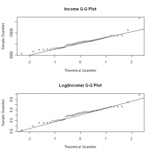
We can also compare q-q plots of the variables:

layout(matrix(1:2,2,2))
qqnorm(cir$income,main=”Income Q-Q Plot”)
qqline(cir$income)
qqnorm(cir$logincome,main=”Log(Income) Q-Q Plot”)
qqline(cir$logincome)

qqplot

For a normally-distributed variable, the q-q plot should appear roughly linear. For a right-skewed variable such as income, the log transformation addresses the higher outliers, and we can see some improvement from examining the upper right of the q-q plot. However, as we have also seen by looking at the box plots, it is sometimes difficult to tell by visual examination alone, and it is useful to get corroboration by running normality tests such as the one shown above (Shapiro-Wilk).
Checking the Match in a Matched Case-Control Study

Sometimes we wish to conduct a study in which we take a population of interest (the treatment group) and match each case to a similar individual sampled from the population which is not undergoing the treatment (the control group). The goal is to find out whether the outcome we wish to measure after treatment is significantly different for each population. This is known as an individually matched case-control study. This post will focus on checking that the matched case population is similar to the control population.

For example, say that we want to find out if providing an incentive to individuals in the treatment group will influence their behavior. We might match on the following variables: medical condition, gender, geographic area, age, risk score, number of office visits in the past 12 months, and total medical cost (TMC) in the past 12 months. Some of these we would want an exact match for (the first 3 variables in this example), whereas the last 4 variables we would match within a given range.

After we run the match, we want to check that the characteristics for the treatment group are similar to those of the control group — that the population means are not significantly different for the continuous variables such as TMC. In order to check this, we first want to test for normality. Whether or not the variable is normally distributed will determine which kind of test we run to see if there is a significant difference between the two groups.

To test normality for the variable TMC, we can use PROC UNIVARIATE as follows:

proc univariate data=work.testdata normal plot;
var TMC;
qqplot TMC /normal(mu=est sigma=est color=red L=1);
run;

This will give you a boxplot and a q-q plot, and the NORMAL option will also give you some normality tests, including Shapiro-Wilk (good for sample sizes < 2000). For normality, you want the mean and the median to be close together on the box plot, a reasonably symmetric distribution (skew close to zero), a relatively straight line for the q-q plot, and the p-values on the normality test results should be > 0.05. If the Shapiro-Wilk W value is close to 1, this also indicates that the data is normal. If p-values are less than 0.05 (alpha), that means you reject the null hypothesis that the distribution is normal and proceed with non-parametric testing.

Assuming your distribution is normal, you would run a paired t-test to see if TMC is similar for both populations (in this example, “study_group” is a flag variable that indicates whether the observation is in the treatment/study group or the control group):

proc ttest data=work.testdata;
paired TMC*study_group;
run;

The null hypothesis is that there is no statistically significant difference between the two groups, so you would want to see a large p-value here (>0.05). This would indicate that our two populations are well-matched on this variable.

However, it is unlikely that TMC is normally distributed, so you would probably end up using the NPAR1WAY procedure instead, with the Wilcoxon test (again, the null hypothesis says that the means are equal, so we want large p-values since we want to accept the null hypothesis):

proc npar1way data=work.testdata wilcoxon;
class study_group;
var TMC;
run;

The tests shown above have all been for continuous variables. Alternatively, if you wanted to test a discrete variable such as gender, you could use PROC FREQ with a chi square test to ensure that gender is independent of the study_group variable:

proc freq data=work.testdata;
tables study_group*male / chisq fisher;
run;